KT AIVLE/Daily Review
240927
bestone888
2024. 9. 29. 21:17
240927
복습
In [4]:
# 보스턴 집값 데이터
import pandas as pd
import numpy as np
import matplotlib.pyplot as plt
import seaborn as sns
import scipy.stats as spst
In [6]:
boston = pd.read_csv('https://raw.githubusercontent.com/DA4BAM/dataset/master/boston.csv')
boston.head()
Out[6]:
crimzninduschasnoxrmagedisradtaxptratiolstatmedv01234
| 0.00632 | 18.0 | 2.31 | 0 | 0.538 | 6.575 | 65.2 | 4.0900 | 1 | 296 | 15.3 | 4.98 | 24.0 |
| 0.02731 | 0.0 | 7.07 | 0 | 0.469 | 6.421 | 78.9 | 4.9671 | 2 | 242 | 17.8 | 9.14 | 21.6 |
| 0.02729 | 0.0 | 7.07 | 0 | 0.469 | 7.185 | 61.1 | 4.9671 | 2 | 242 | 17.8 | 4.03 | 34.7 |
| 0.03237 | 0.0 | 2.18 | 0 | 0.458 | 6.998 | 45.8 | 6.0622 | 3 | 222 | 18.7 | 2.94 | 33.4 |
| 0.06905 | 0.0 | 2.18 | 0 | 0.458 | 7.147 | 54.2 | 6.0622 | 3 | 222 | 18.7 | 5.33 | 36.2 |
In [11]:
# crim(범죄율) -> medv(집값) 시각화, 수치화

sns.scatterplot(x = 'crim', y = 'medv', data = boston)
plt.grid()
plt.show()

In [13]:
temp = boston.loc[boston['crim'].notnull()]

spst.pearsonr(temp['crim'], temp['medv'])
Out[13]:
PearsonRResult(statistic=-0.3883046085868116, pvalue=1.1739870821943826e-19)In [17]:
# 음의 상관관계
# mdev 50 에 몰린 이유는 설문조사의 최댓값이 50이기 때문일 것이다
In [21]:
# tax(제산세율) -> medv(집값) 시각화, 수치화
sns.scatterplot(x = 'tax', y = 'medv', data = boston)
plt.grid()
plt.show()

In [25]:
temp = boston.loc[boston['tax'].notnull()]
spst.pearsonr(temp['tax'], temp['medv'])
Out[25]:
PearsonRResult(statistic=-0.4685359335677671, pvalue=5.637733627690444e-29)In [28]:
# 음의 상관관계
In [33]:
# tax(제산세율) -> medv(집값) 시각화, 수치화
# tax의 500 이상인 값은 제거하고 다시 수행

temp = boston.loc[boston['tax']<500]
spst.pearsonr(temp['tax'], temp['medv'])
Out[33]:
PearsonRResult(statistic=-0.2923180757786092, pvalue=1.0549678915090099e-08)In [35]:
# tax 500 이상인 값이 상관계수 -0.46에 영향을 크게 미침
In [39]:
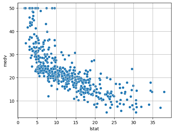
# lstat(하위계층비율) -> medv(집값) 시각화, 수치화
sns.scatterplot(x = 'lstat', y = 'medv', data= boston)
plt.grid()
plt.show()
In [41]:
temp = boston.loc[boston['lstat'].notnull()]
spst.pearsonr(temp['lstat'], temp['medv'])
Out[41]:
PearsonRResult(statistic=-0.7376627261740148, pvalue=5.081103394387554e-88)In [43]:
# 강한 음의 상관관계
In [51]:
# ptratio(교사 1명당 학생 수) -> medv(집값) 시각화, 수치화
sns.scatterplot(x ='ptratio', y = 'medv', data = boston)
plt.grid()
plt.show()


In [55]:
# 범주 내에선 규칙이 없어 보이지만, 범주 간에는 있어 보임
In [57]:
# 전체 변수간 상관관계
boston.corr()
Out[57]:
crimzninduschasnoxrmagedisradtaxptratiolstatmedvcrimzninduschasnoxrmagedisradtaxptratiolstatmedv
| 1.000000 | -0.200469 | 0.406583 | -0.055892 | 0.420972 | -0.219247 | 0.352734 | -0.379670 | 0.625505 | 0.582764 | 0.289946 | 0.455621 | -0.388305 |
| -0.200469 | 1.000000 | -0.533828 | -0.042697 | -0.516604 | 0.311991 | -0.569537 | 0.664408 | -0.311948 | -0.314563 | -0.391679 | -0.412995 | 0.360445 |
| 0.406583 | -0.533828 | 1.000000 | 0.062938 | 0.763651 | -0.391676 | 0.644779 | -0.708027 | 0.595129 | 0.720760 | 0.383248 | 0.603800 | -0.483725 |
| -0.055892 | -0.042697 | 0.062938 | 1.000000 | 0.091203 | 0.091251 | 0.086518 | -0.099176 | -0.007368 | -0.035587 | -0.121515 | -0.053929 | 0.175260 |
| 0.420972 | -0.516604 | 0.763651 | 0.091203 | 1.000000 | -0.302188 | 0.731470 | -0.769230 | 0.611441 | 0.668023 | 0.188933 | 0.590879 | -0.427321 |
| -0.219247 | 0.311991 | -0.391676 | 0.091251 | -0.302188 | 1.000000 | -0.240265 | 0.205246 | -0.209847 | -0.292048 | -0.355501 | -0.613808 | 0.695360 |
| 0.352734 | -0.569537 | 0.644779 | 0.086518 | 0.731470 | -0.240265 | 1.000000 | -0.747881 | 0.456022 | 0.506456 | 0.261515 | 0.602339 | -0.376955 |
| -0.379670 | 0.664408 | -0.708027 | -0.099176 | -0.769230 | 0.205246 | -0.747881 | 1.000000 | -0.494588 | -0.534432 | -0.232471 | -0.496996 | 0.249929 |
| 0.625505 | -0.311948 | 0.595129 | -0.007368 | 0.611441 | -0.209847 | 0.456022 | -0.494588 | 1.000000 | 0.910228 | 0.464741 | 0.488676 | -0.381626 |
| 0.582764 | -0.314563 | 0.720760 | -0.035587 | 0.668023 | -0.292048 | 0.506456 | -0.534432 | 0.910228 | 1.000000 | 0.460853 | 0.543993 | -0.468536 |
| 0.289946 | -0.391679 | 0.383248 | -0.121515 | 0.188933 | -0.355501 | 0.261515 | -0.232471 | 0.464741 | 0.460853 | 1.000000 | 0.374044 | -0.507787 |
| 0.455621 | -0.412995 | 0.603800 | -0.053929 | 0.590879 | -0.613808 | 0.602339 | -0.496996 | 0.488676 | 0.543993 | 0.374044 | 1.000000 | -0.737663 |
| -0.388305 | 0.360445 | -0.483725 | 0.175260 | -0.427321 | 0.695360 | -0.376955 | 0.249929 | -0.381626 | -0.468536 | -0.507787 | -0.737663 | 1.000000 |
In [ ]:
표준오차
- 표본평균과 모평균은 일치하지 않을 수 있음
95% 신뢰구간
- 표본평균을 100개 추출했을 때 95개는 모평균을 포함함
In [92]:
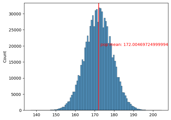
# 임의의 모집단 만들기
import random as rd

# 평균 172, 표준편차 7인 정규분포 내에서 랜덤변수 생성
pop = [round(rd.normalvariate(172, 7),1) for i in range(800000)]

sns.histplot(pop, bins = 100)
plt.axvline(np.mean(pop), color = 'r')

# 텍스트 입력
# plt.text(x좌표, y좌표, 쓸 내용)
plt.text(np.mean(pop)+1, 20000,'pop mean: {}'.format(np.mean(pop)), color = 'r')

plt.show()
In [94]:
# 표본크기 50인 표본 100개뽑기
x_mean = []
for i in range(100):
    s1 = rd.sample(pop, 50)
    s1 = pd.Series(s1)
    x_mean.append(round(s1.mean(), 3))

x_mean
Out[94]:
[172.032,
 172.288,
 172.162,
 171.622,
 172.16,
 172.78,
 170.654,
 171.838,
 172.938,
 170.974,
 171.596,
 172.774,
 171.802,
 171.482,
 172.32,
 172.7,
 172.232,
 172.932,
 171.266,
 172.512,
 171.294,
 172.092,
 172.092,
 171.78,
 170.836,
 171.962,
 172.732,
 172.332,
 172.18,
 172.424,
 171.15,
 171.926,
 173.336,
 172.594,
 171.72,
 174.144,
 172.196,
 171.596,
 172.046,
 171.422,
 171.622,
 171.822,
 171.428,
 173.708,
 171.014,
 170.964,
 171.62,
 172.34,
 172.092,
 171.642,
 171.67,
 171.666,
 172.046,
 172.132,
 170.514,
 172.032,
 172.644,
 171.748,
 172.918,
 171.634,
 172.72,
 171.85,
 172.33,
 172.212,
 174.018,
 171.48,
 173.02,
 172.518,
 170.944,
 171.506,
 172.828,
 171.578,
 171.078,
 171.902,
 170.608,
 173.654,
 172.608,
 173.046,
 171.49,
 171.378,
 171.572,
 170.89,
 171.626,
 172.324,
 172.716,
 171.122,
 170.758,
 170.196,
 171.326,
 174.248,
 170.052,
 174.096,
 172.128,
 172.362,
 171.728,
 172.494,
 172.52,
 173.172,
 172.536,
 172.086]
In [109]:
sns.kdeplot(x_mean)
plt.axvline(np.mean(x_mean), color = 'r')
plt.text(np.mean(x_mean)+1, 0.1, 'pop mean {}'.format(round(np.mean(x_mean)),3), color = 'r')
plt.show()

In [113]:
# 모평균 != 표본평균의 평균
# but 유사함

범주 vs 숫자
In [127]:
# 타이타닉 데이터
titanic = pd.read_csv('https://raw.githubusercontent.com/DA4BAM/dataset/master/titanic.0.csv')
titanic.head()
Out[127]:
PassengerIdSurvivedPclassNameSexAgeSibSpParchTicketFareCabinEmbarked01234
| 1 | 0 | 3 | Braund, Mr. Owen Harris | male | 22.0 | 1 | 0 | A/5 21171 | 7.2500 | NaN | S |
| 2 | 1 | 1 | Cumings, Mrs. John Bradley (Florence Briggs Th... | female | 38.0 | 1 | 0 | PC 17599 | 71.2833 | C85 | C |
| 3 | 1 | 3 | Heikkinen, Miss. Laina | female | 26.0 | 0 | 0 | STON/O2. 3101282 | 7.9250 | NaN | S |
| 4 | 1 | 1 | Futrelle, Mrs. Jacques Heath (Lily May Peel) | female | 35.0 | 1 | 0 | 113803 | 53.1000 | C123 | S |
| 5 | 0 | 3 | Allen, Mr. William Henry | male | 35.0 | 0 | 0 | 373450 | 8.0500 | NaN | S |
In [131]:
sns.barplot(x = 'Survived', y = 'Age', data = titanic)
plt.grid()
plt.show()

In [135]:
sns.boxplot(x = 'Survived', y = 'Age', data= titanic)
plt.grid()
plt.show()

수치화
- t test : spst.ttest_ind()
- ANOVA : spst.f_oneway()
t-test : 2 범주
- 두 평균 차이를 표준오차로 나눈 값
- feature, target 사이의 관계 파악
- df.notnull()로 NaN 제거
- t값이 2보다 크거나 -2보다 작으면 차이가 있다
In [155]:
# Survived(범주) -> Age(숫자)

# NaN 값 제거
temp = titanic.loc[titanic['Age'].notnull()]

# 생존자의 Age
survived = temp.loc[temp['Survived'] == 1, 'Age']

# 사망자의 Age
died = temp.loc[temp['Survived'] == 0, 'Age']
In [157]:
# t-test
spst.ttest_ind(survived, died)
Out[157]:
TtestResult(statistic=-2.06668694625381, pvalue=0.03912465401348249, df=712.0)In [159]:
# Sex(범주) -> Fare(숫자)

# 남성의 Fare
m = titanic.loc[titanic['Sex'] == 'male', 'Fare']

# 여성의 Fare
f = titanic.loc[titanic['Sex'] == 'female', 'Fare']

# t-test
spst.ttest_ind(m, f)
Out[159]:
TtestResult(statistic=-5.529140269385719, pvalue=4.2308678700429995e-08, df=889.0)ANOVA : 3 범주 이상
In [164]:
# Pclass(범주) -> Age(숫자)

# NaN 제거
temp = titanic.loc[titanic['Age'].notnull()]

# 클래스1
p1 = temp.loc[temp['Pclass'] == 1, 'Age']
p2 = temp.loc[temp['Pclass'] == 2, 'Age']
p3 = temp.loc[temp['Pclass'] == 3, 'Age']

# ANOVA
spst.f_oneway(p1, p2, p3)
Out[164]:
F_onewayResult(statistic=57.443484340676214, pvalue=7.487984171959904e-24)In [ ]: