KT AIVLE/Daily Review
241021 ~ 241022
bestone888
2024. 10. 28. 01:18
241021 ~ 241022
비지도 학습
- 차원축소
- 클러스터링
- 이상탐지
In [177]:
import pandas as pd
import numpy as np
import matplotlib.pyplot as plt
import seaborn as sns

from sklearn.model_selection import train_test_split
from sklearn.neighbors import KNeighborsClassifier
from sklearn.metrics import *

from sklearn.datasets import load_breast_cancer, load_digits, load_iris, make_swiss_roll
from sklearn.preprocessing import MinMaxScaler

from sklearn.decomposition import PCA
1. PCA
In [179]:
iris = pd.read_csv("https://raw.githubusercontent.com/DA4BAM/dataset/master/iris.csv")
target = 'Species'
x = iris.drop(target, axis = 1)
y = iris.loc[:, target]
x.tail()
Out[179]:
Sepal.LengthSepal.WidthPetal.LengthPetal.Width145146147148149
| 6.7 | 3.0 | 5.2 | 2.3 |
| 6.3 | 2.5 | 5.0 | 1.9 |
| 6.5 | 3.0 | 5.2 | 2.0 |
| 6.2 | 3.4 | 5.4 | 2.3 |
| 5.9 | 3.0 | 5.1 | 1.8 |
In [180]:
# 스케일링
scaler = MinMaxScaler()
x2 = scaler.fit_transform(x)
x2[:10]
Out[180]:
array([[0.22222222, 0.625     , 0.06779661, 0.04166667],
       [0.16666667, 0.41666667, 0.06779661, 0.04166667],
       [0.11111111, 0.5       , 0.05084746, 0.04166667],
       [0.08333333, 0.45833333, 0.08474576, 0.04166667],
       [0.19444444, 0.66666667, 0.06779661, 0.04166667],
       [0.30555556, 0.79166667, 0.11864407, 0.125     ],
       [0.08333333, 0.58333333, 0.06779661, 0.08333333],
       [0.19444444, 0.58333333, 0.08474576, 0.04166667],
       [0.02777778, 0.375     , 0.06779661, 0.04166667],
       [0.16666667, 0.45833333, 0.08474576, 0.        ]])
In [181]:
# x2를 데이터프레임으로 변환
x2 = pd.DataFrame(x2, columns = x.columns)
In [182]:
x2.tail()
Out[182]:
Sepal.LengthSepal.WidthPetal.LengthPetal.Width145146147148149
| 0.666667 | 0.416667 | 0.711864 | 0.916667 |
| 0.555556 | 0.208333 | 0.677966 | 0.750000 |
| 0.611111 | 0.416667 | 0.711864 | 0.791667 |
| 0.527778 | 0.583333 | 0.745763 | 0.916667 |
| 0.444444 | 0.416667 | 0.694915 | 0.708333 |
In [183]:
from sklearn.decomposition import PCA
In [184]:
# 열 개수 확인
x2.shape[1]
Out[184]:
4In [185]:
# 주성분 개수 (2개)
n = 2
pca = PCA(n_components = n)

x2_pc = pca.fit_transform(x2)

# 데이터프레임 변환
x2_pc = pd.DataFrame(x2_pc, columns = ['PC1','PC2'])

# 확인
x2_pc.tail()
Out[185]:
PC1PC2145146147148149
| 0.551462 | 0.059841 |
| 0.407146 | -0.171821 |
| 0.447143 | 0.037560 |
| 0.488208 | 0.149678 |
| 0.312066 | -0.031130 |
In [186]:
# 시각화
sns.scatterplot(x = 'PC1', y = 'PC2', data = x2_pc, hue = y)
plt.grid()
plt.show()
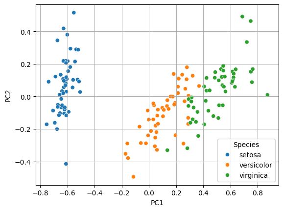
1-1. PCA: 고차원 데이터 축소
In [188]:
cancer=load_breast_cancer()
x = cancer.data
y = cancer.target

x = pd.DataFrame(x, columns=cancer.feature_names)
In [189]:
# 열 개수 확인
x.shape[1]
Out[189]:
30In [190]:
# 스케일링
scaler = MinMaxScaler()
x = scaler.fit_transform(x)

# 데이터프레임
x = pd.DataFrame(x)
x.tail()
Out[190]:
0123456789...20212223242526272829564565566567568
| 0.690000 | 0.428813 | 0.678668 | 0.566490 | 0.526948 | 0.296055 | 0.571462 | 0.690358 | 0.336364 | 0.132056 | ... | 0.623266 | 0.383262 | 0.576174 | 0.452664 | 0.461137 | 0.178527 | 0.328035 | 0.761512 | 0.097575 | 0.105667 |
| 0.622320 | 0.626987 | 0.604036 | 0.474019 | 0.407782 | 0.257714 | 0.337395 | 0.486630 | 0.349495 | 0.113100 | ... | 0.560655 | 0.699094 | 0.520892 | 0.379915 | 0.300007 | 0.159997 | 0.256789 | 0.559450 | 0.198502 | 0.074315 |
| 0.455251 | 0.621238 | 0.445788 | 0.303118 | 0.288165 | 0.254340 | 0.216753 | 0.263519 | 0.267677 | 0.137321 | ... | 0.393099 | 0.589019 | 0.379949 | 0.230731 | 0.282177 | 0.273705 | 0.271805 | 0.487285 | 0.128721 | 0.151909 |
| 0.644564 | 0.663510 | 0.665538 | 0.475716 | 0.588336 | 0.790197 | 0.823336 | 0.755467 | 0.675253 | 0.425442 | ... | 0.633582 | 0.730277 | 0.668310 | 0.402035 | 0.619626 | 0.815758 | 0.749760 | 0.910653 | 0.497142 | 0.452315 |
| 0.036869 | 0.501522 | 0.028540 | 0.015907 | 0.000000 | 0.074351 | 0.000000 | 0.000000 | 0.266162 | 0.187026 | ... | 0.054287 | 0.489072 | 0.043578 | 0.020497 | 0.124084 | 0.036043 | 0.000000 | 0.000000 | 0.257441 | 0.100682 |
5 rows × 30 columns
In [191]:
# train, val 분할
x_train, x_val, y_train, y_val = train_test_split(x, y, stratify = y, test_size = 0.3, random_state = 1)
In [192]:
# 주성분 개수 결정(열 개수)
n = x_train.shape[1]

# 주성분 분석
pca = PCA(n_components=n)

# 만들고 적용
x_train_pc = pca.fit_transform(x_train)
x_val_pc = pca.transform(x_val)

# 데이터프레임 변환
x_train_pc = pd.DataFrame(x_train_pc)
x_val_pc = pd.DataFrame(x_val_pc)

# 확인
x_train_pc.tail()
Out[192]:
0123456789...20212223242526272829393394395396397
| 0.604496 | 0.293004 | -0.116841 | 0.090776 | 0.174731 | 0.094767 | -0.152215 | -0.040985 | 0.004279 | 0.074266 | ... | 0.016156 | -0.012057 | -0.021115 | -0.019502 | -0.001542 | -0.000116 | -0.010140 | 0.004784 | 0.000520 | 0.001084 |
| 0.670441 | 0.404470 | 0.276673 | -0.039954 | -0.005364 | -0.214431 | -0.145094 | 0.005926 | -0.102698 | 0.046341 | ... | 0.020150 | -0.002203 | -0.012603 | -0.025600 | -0.016966 | 0.021131 | 0.005030 | 0.006541 | 0.008435 | -0.000204 |
| -0.422708 | 0.082693 | -0.336754 | -0.266818 | 0.003538 | -0.037045 | 0.005500 | 0.113135 | -0.010462 | 0.016478 | ... | -0.034630 | 0.010318 | 0.001375 | -0.006140 | 0.014824 | -0.009868 | -0.007537 | 0.000381 | 0.001833 | 0.002374 |
| -0.348721 | -0.225762 | 0.172474 | -0.023669 | -0.029797 | -0.151742 | -0.010541 | -0.029293 | -0.085196 | -0.037646 | ... | 0.028259 | -0.015652 | -0.001355 | 0.000464 | -0.011440 | 0.008870 | 0.002034 | -0.000491 | 0.001360 | -0.000684 |
| 0.471659 | -0.457314 | -0.371755 | 0.326655 | 0.084525 | 0.045097 | -0.113786 | 0.136283 | -0.138986 | -0.073532 | ... | 0.017423 | -0.079871 | 0.004645 | 0.033389 | 0.034341 | -0.006584 | 0.011966 | -0.009223 | -0.000625 | 0.001437 |
5 rows × 30 columns
In [193]:
x_val_pc
Out[193]:
0123456789...2021222324252627282901234...166167168169170
| 0.986466 | -0.235670 | 0.270415 | 0.092429 | 0.086037 | -0.033833 | 0.197333 | -0.119268 | -0.074422 | -0.037586 | ... | 0.013571 | -0.024155 | 0.018648 | 0.017538 | -0.006876 | -0.059477 | -0.014808 | -0.002047 | 0.002373 | 0.009680 |
| -0.104579 | -0.074307 | 0.312840 | 0.099448 | 0.011891 | -0.152601 | -0.013334 | -0.085877 | -0.103034 | -0.035206 | ... | 0.030758 | -0.012674 | -0.015146 | 0.001926 | 0.015507 | -0.016077 | -0.001161 | 0.005877 | 0.000121 | -0.000560 |
| -0.606859 | 0.057073 | 0.079678 | 0.216490 | -0.105960 | -0.008291 | -0.016352 | -0.035527 | 0.000446 | 0.109191 | ... | 0.008037 | -0.046095 | 0.022887 | -0.011350 | -0.001340 | -0.002501 | -0.006813 | 0.006396 | -0.002151 | -0.001550 |
| 0.826971 | -0.213466 | 0.170124 | 0.158292 | -0.048970 | 0.297659 | -0.187783 | 0.004894 | -0.130852 | 0.014084 | ... | -0.015564 | -0.006216 | 0.000906 | -0.014260 | -0.016040 | -0.014097 | 0.010106 | -0.007289 | 0.000391 | -0.002170 |
| 0.289178 | -0.106043 | -0.079450 | -0.142993 | -0.122178 | -0.064969 | -0.101990 | 0.019891 | 0.111451 | 0.022634 | ... | 0.004606 | -0.007942 | -0.021379 | 0.009283 | 0.000165 | -0.001646 | -0.000317 | 0.006153 | -0.005273 | 0.000916 |
| ... | ... | ... | ... | ... | ... | ... | ... | ... | ... | ... | ... | ... | ... | ... | ... | ... | ... | ... | ... | ... |
| -0.788188 | -0.071533 | -0.087170 | 0.199220 | -0.147930 | 0.192540 | 0.046487 | -0.018149 | -0.013533 | 0.107620 | ... | -0.004893 | 0.047330 | 0.021252 | 0.005843 | -0.024457 | 0.003811 | -0.000996 | 0.000044 | 0.001602 | 0.001613 |
| 0.350618 | -0.632874 | -0.154034 | 0.056093 | 0.040454 | 0.212023 | -0.055636 | -0.025029 | 0.031029 | 0.006190 | ... | -0.012841 | 0.003694 | 0.001127 | 0.004568 | 0.011472 | 0.001291 | 0.011151 | -0.004585 | -0.004109 | -0.001843 |
| -0.643508 | -0.487221 | -0.090474 | -0.039606 | 0.195281 | 0.119339 | 0.035837 | -0.065802 | 0.036939 | 0.047342 | ... | -0.004344 | 0.000743 | 0.001916 | -0.007648 | -0.005007 | 0.016565 | -0.007999 | 0.002791 | 0.000808 | -0.002943 |
| 1.005517 | 1.501756 | -0.029630 | -0.150702 | -0.239054 | 0.390628 | 0.246087 | 0.009406 | -0.221912 | 0.114488 | ... | -0.042372 | 0.040525 | 0.020705 | 0.003518 | -0.041782 | 0.061190 | 0.020887 | 0.004298 | -0.010684 | -0.005676 |
| 0.628945 | 0.473751 | 0.362178 | -0.291157 | -0.024450 | 0.109613 | 0.138980 | -0.006914 | 0.089684 | -0.017310 | ... | -0.035056 | -0.040647 | 0.031005 | -0.017225 | 0.010369 | -0.020221 | -0.014892 | -0.010807 | 0.004997 | 0.001298 |
171 rows × 30 columns
In [194]:
# 주성분 1개짜리
pca1 = PCA(n_components=1)
x_train_pc1 = pca1.fit_transform(x_train)
In [195]:
# 주성분 2개짜리
pca2 = PCA(n_components = 2)
x_train_pc2 = pca2.fit_transform(x_train)
In [196]:
# 주성분 3개짜리
pca3 = PCA(n_components = 3)
x_train_pc3 = pca3.fit_transform(x_train)
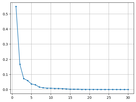
In [197]:
# 각 주성분이 데이터 정보를 얼마나 담고 있는지
# 시각화
plt.plot(range(1, n+1), pca.explained_variance_ratio_, marker = '.')
plt.grid()
plt.show()
In [221]:
# 상위 2개 시각화
sns.scatterplot(x = 0, y = 1, data = x_train_pc, hue = y_train)
plt.grid()
plt.show()
In [ ]:
2. k-means
In [260]:
import pandas as pd
import numpy as np
from matplotlib import pyplot as plt
import seaborn as sns

# 샘플데이터 로딩 함수
from sklearn.datasets import make_blobs, make_moons

# 클러스터링을 위한 함수
from sklearn.neighbors import NearestNeighbors
from sklearn.cluster import KMeans, DBSCAN

import warnings
warnings.filterwarnings("ignore", category=UserWarning)
In [264]:
x, y = make_blobs(n_samples=300, centers=4, cluster_std=0.60, random_state=0)
x = pd.DataFrame(x, columns = ['x1', 'x2'])
y = pd.Series(y, name = 'shape')

plt.figure(figsize = (6,4))
plt.scatter(x['x1'], x['x2'])
plt.show()
In [266]:
# k-means 학습
model = KMeans(n_clusters = 2, n_init = 'auto')
model.fit(x)

# 예측
pred = model.predict(x)
print(pred)
[0 1 0 1 0 0 0 0 1 1 0 1 0 1 0 0 0 0 0 0 0 0 0 0 0 0 0 0 0 0 1 1 0 1 1 1 1
 1 0 0 0 0 1 0 0 0 1 0 1 0 0 0 1 0 0 0 1 0 1 0 1 0 1 0 0 0 1 0 1 0 0 0 1 0
 0 1 0 0 0 1 0 0 0 0 1 0 0 0 1 1 0 0 1 0 0 0 0 0 1 0 1 0 1 0 0 0 0 0 1 0 0
 0 0 1 0 0 1 0 0 0 0 0 0 0 0 0 0 0 0 0 1 0 0 0 1 0 0 1 0 1 1 0 0 0 0 0 1 0
 1 1 1 0 1 0 0 0 1 0 0 0 1 0 0 0 0 0 0 0 0 0 0 1 0 0 0 1 0 0 0 0 0 0 0 0 0
 0 0 0 0 1 0 0 0 0 0 0 0 0 0 1 0 0 0 0 0 1 0 1 0 1 0 0 0 0 1 0 0 0 0 0 1 0
 0 0 0 0 0 1 1 0 0 1 0 0 0 0 0 0 1 0 0 0 0 1 1 1 1 0 0 1 0 0 0 0 0 0 0 0 0
 1 0 0 0 0 1 0 0 1 0 0 0 0 0 0 0 0 0 0 1 1 0 0 0 0 0 0 1 0 1 0 0 0 1 1 1 0
 0 0 1 0]
In [269]:
# pred 데이터프레임 만들기
pred = pd.DataFrame(pred, columns = ['Predicted'])
result = pd.concat([x, pred, y], axis = 1)
result.head()
Out[269]:
x1x2Predictedshape01234
| 0.836857 | 2.136359 | 0 | 1 |
| -1.413658 | 7.409623 | 1 | 3 |
| 1.155213 | 5.099619 | 0 | 0 |
| -1.018616 | 7.814915 | 1 | 3 |
| 1.271351 | 1.892542 | 0 | 1 |
In [276]:
# 결과 시각화
centers = pd.DataFrame(model.cluster_centers_, columns = ['x1', 'x2'])
centers
Out[276]:
x1x201
| 0.452332 | 2.681056 |
| -1.334654 | 7.694427 |
In [283]:
plt.scatter(result['x1'], result['x2'], c = result['Predicted'], alpha = 0.5)
plt.scatter(centers['x1'], centers['x2'], c = 'r')
plt.show()
In [287]:
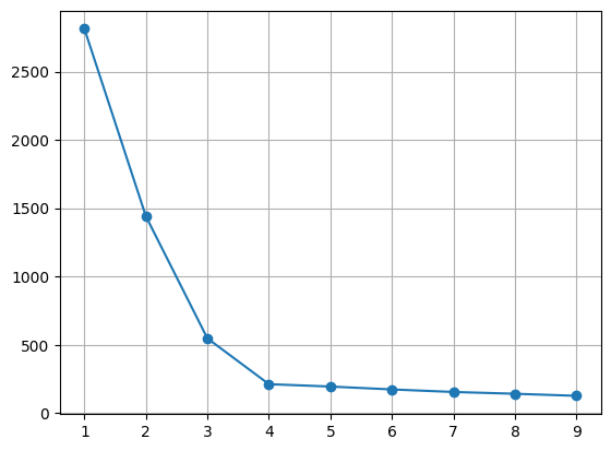
# 적절한 k값 찾기 (inertia)

# inertia -> k 결정
model.inertia_
Out[287]:
1190.7823593643448In [291]:
kvalues = range(1, 10)
inertias = list()

for k in kvalues:
    model = KMeans(n_clusters= k, n_init = 'auto')
    model.fit(x)
    inertias.append(model.inertia_)


# 시각화
plt.plot(range(1,10), inertias, marker = 'o')
plt.grid()
plt.show()
In [294]:
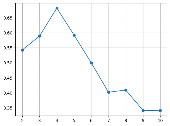
# 적절한 k값 찾기 (silhouette score)
from sklearn.metrics import silhouette_score

kvalues = range(2, 11)
sil_score = list()

for k in kvalues:
    model = KMeans(n_clusters= k , n_init = 'auto')

    pred = model.fit_predict(x)
    sil_score.append(silhouette_score(x, pred))


# 시각화
plt.plot(kvalues, sil_score, marker = 'o')
plt.grid()
plt.show()
2-1. k-means
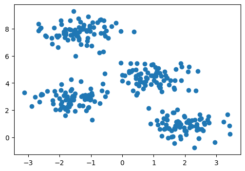
In [304]:
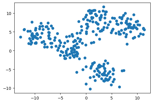
# 데이터
x, y = make_blobs(n_samples=300, centers=5, cluster_std=1.8, random_state=20)
x = pd.DataFrame(x, columns = ['x1', 'x2'])
y = pd.Series(y, name = 'shape')

plt.figure(figsize = (6,4))
plt.scatter(x['x1'], x['x2'])
plt.show()
In [306]:
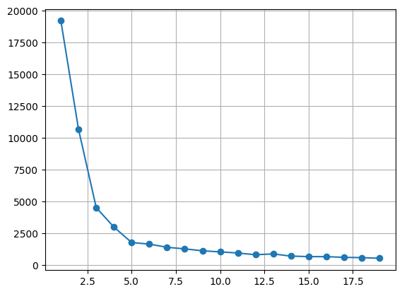
# 1. inertia
In [313]:
kvalues = range(1, 20)
inertias = list()

for k in kvalues:
    model = KMeans(n_clusters = k, n_init = 'auto')
    model.fit(x)
    inertias.append(model.inertia_)

# 시각화
plt.plot(kvalues, inertias, marker = 'o')
plt.grid()
plt.show()
In [315]:
# 2. silhouette score
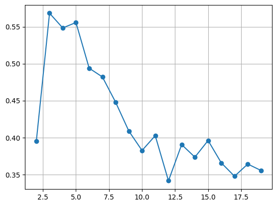
In [319]:
kvalues = range(2, 20)
sil_score = list()

for k in kvalues:
    model = KMeans(n_clusters = k, n_init = 'auto')
    pred = model.fit_predict(x)
    sil_score.append(silhouette_score(x, pred))

# 시각화
plt.plot(kvalues, sil_score, marker = 'o')
plt.grid()
plt.show()
In [ ]:
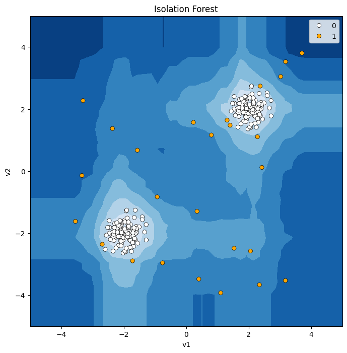
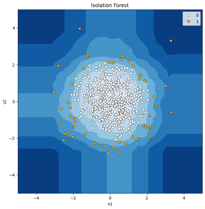
3. Isolation Forest
In [337]:
import pandas as pd
import numpy as np
import matplotlib.pyplot as plt
import seaborn as sns

from sklearn.model_selection import train_test_split
from sklearn.ensemble import IsolationForest # Isolation Forest!
from sklearn.metrics import *

from tqdm import tqdm
import warnings
warnings.simplefilter(action='ignore')
In [339]:
# Single Blob
X1 = pd.read_csv('https://raw.githubusercontent.com/DA4BAM/dataset/master/Anomaly_X.csv')

# Double Blob
X2 = pd.read_csv('https://raw.githubusercontent.com/DA4BAM/dataset/master/Anomaly_X2.csv')
In [340]:
# 함수 불러오기

def model_visualize(model, v1, v2, title = "") :
    # 메쉬그리드값 저장하기
    xx, yy = np.meshgrid(np.linspace(-5, 5, 50), np.linspace(-5, 5, 50)) # mesh grid

    # 메쉬 그리드값에 대해 모델 부터 Anomaly Score 만들기.
    Z = model.decision_function(np.c_[xx.ravel(), yy.ravel()]) # Anomaly Score
    Z = Z.reshape(xx.shape)
    # 시각화
    plt.figure(figsize = (8,8))
    plt.title(title)

    # 메쉬그리드 값의 Anomaly Score에 대한 등고선
    plt.contourf(xx, yy, Z, cmap=plt.cm.Blues_r)

    # 데이터 산점도 그리기.(예측 결과 Abnormal은 오렌지색, Normal은 흰색)
    sns.scatterplot(x=v1, y=v2, sizes = 30, edgecolor='k', hue = pred, palette=['white', 'orange'])

    plt.axis("tight")
    plt.xlim(-5, 5)
    plt.ylim(-5, 5)
    plt.show()
In [346]:
# Single Blob
# isolation forest 모델
model = IsolationForest(contamination= 0.1, n_estimators= 50)    # 입력저오의 0.1을 비정상으로 처리, tree 50개
model.fit(X1)
pred = model.predict(X1)
pred = np.where(pred ==1, 0 ,1)

# 시각화
model_visualize(model, X1['v1'], X1['v2'], 'Isolation Forest')
In [349]:
# Double Blob
# isolation forest

model = IsolationForest(contamination = 0.1, n_estimators = 50 )
model.fit(X2)
pred = model.predict(X2)
pred = np.where(pred == 1, 0, 1)

model_visualize(model, X2['v1'],X2['v2'], 'Isolation Forest')