241015

241015

회귀 성능 평가

In [8]:

import numpy as np
import pandas as pd
import matplotlib.pyplot as plt
import seaborn as sns
import warnings

warnings.filterwarnings(action='ignore')
%config InlineBackend.figure_format = 'retina'

In [11]:

path = 'https://raw.githubusercontent.com/Jangrae/csv/master/airquality_simple.csv'
data = pd.read_csv(path)

In [19]:

data.tail()

Out[19]:

OzoneSolar.RWindTempMonthDay148149150151152

30	193.0	6.9	70	9	26
23	145.0	13.2	77	9	27
14	191.0	14.3	75	9	28
18	131.0	8.0	76	9	29
20	223.0	11.5	68	9	30

In [21]:

data.info()

<class 'pandas.core.frame.DataFrame'>
RangeIndex: 153 entries, 0 to 152
Data columns (total 6 columns):
 #   Column   Non-Null Count  Dtype  
---  ------   --------------  -----  
 0   Ozone    153 non-null    int64  
 1   Solar.R  146 non-null    float64
 2   Wind     153 non-null    float64
 3   Temp     153 non-null    int64  
 4   Month    153 non-null    int64  
 5   Day      153 non-null    int64  
dtypes: float64(2), int64(4)
memory usage: 7.3 KB

In [23]:

data['Solar.R'].ffill(inplace = True)

In [37]:

from sklearn.model_selection import train_test_split
x = data.drop(columns = 'Ozone')
y = data['Ozone']

x_train, x_test, y_train, y_test = train_test_split(x, y, test_size = 0.3, random_state = 1)

In [48]:

from sklearn.linear_model import LinearRegression

model = LinearRegression()

In [50]:

model.fit(x_train, y_train)

Out[50]:

  LinearRegression?i

LinearRegression()

In [52]:

y_pred = model.predict(x_test)

In [54]:

# MAE: mean absolute error
from sklearn.metrics import mean_absolute_error

mean_absolute_error(y_test, y_pred)

Out[54]:

13.15711939503116

In [56]:

# MSE: mean squared error
from sklearn.metrics import mean_squared_error

mean_squared_error(y_test, y_pred)

Out[56]:

313.51536709100935

In [58]:

# RMSE: root mean squared error
from sklearn.metrics import root_mean_squared_error

root_mean_squared_error(y_test, y_pred)

Out[58]:

17.70636515750789

In [60]:

# MAPE: mean absolute percentage error
from sklearn.metrics import mean_absolute_percentage_error

mean_absolute_percentage_error(y_test, y_pred)

Out[60]:

0.43772048098386984

In [62]:

# R2-score
from sklearn.metrics import r2_score

r2_score(y_test, y_pred)

Out[62]:

0.6094929125427131

분류 성능 평가

In [66]:

path = 'https://raw.githubusercontent.com/Jangrae/csv/master/admission_simple.csv'
data = pd.read_csv(path)

In [68]:

data.tail()

Out[68]:

GRETOEFLRANKSOPLORGPARESEARCHADMIT495496497498499

332	108	5	4.5	4.0	9.02	1	1
337	117	5	5.0	5.0	9.87	1	1
330	120	5	4.5	5.0	9.56	1	1
312	103	4	4.0	5.0	8.43	0	0
327	113	4	4.5	4.5	9.04	0	1

In [70]:

target = 'ADMIT'

x = data.drop(columns = target)
y = data[target]

In [74]:

from sklearn.model_selection import train_test_split

x_train, x_test, y_train, y_test = train_test_split(x, y,
                                                   stratify =y,
                                                   test_size = 0.3,
                                                   random_state = 1)

In [76]:

from sklearn.neighbors import KNeighborsClassifier

model = KNeighborsClassifier()
model.fit(x_train, y_train)
y_pred = model.predict(x_test)

In [95]:

# Confusion Mmatrix
from sklearn.metrics import confusion_matrix
confusion_matrix(y_test, y_pred)

Out[95]:

array([[76,  9],
       [14, 51]], dtype=int64)

In [109]:

plt.figure(figsize = (5,5))
sns.heatmap(confusion_matrix(y_test, y_pred),
           annot = True,
           fmt = '.2f',
           cbar = False,
           cmap = 'Blues')
plt.show()

In [111]:

# Accuracy
from sklearn.metrics import accuracy_score

accuracy_score(y_test, y_pred)

Out[111]:

0.8466666666666667

In [113]:

# Precision
from sklearn.metrics import precision_score

precision_score(y_test, y_pred)

Out[113]:

0.85

In [115]:

# Recall
from sklearn.metrics import recall_score

recall_score(y_test, y_pred)

Out[115]:

0.7846153846153846

In [120]:

# F1-Score
from sklearn.metrics import f1_score

f1_score(y_test, y_pred)

Out[120]:

0.816

In [122]:

# Classification Report
from sklearn.metrics import classification_report

print(classification_report(y_test, y_pred))

              precision    recall  f1-score   support

           0       0.84      0.89      0.87        85
           1       0.85      0.78      0.82        65

    accuracy                           0.85       150
   macro avg       0.85      0.84      0.84       150
weighted avg       0.85      0.85      0.85       150

In [ ]:

선형회귀

In [128]:

path = 'https://raw.githubusercontent.com/Jangrae/csv/master/cars.csv'
data = pd.read_csv(path)

In [134]:

data.head()

Out[134]:

speeddist01234

4	2
4	10
7	4
7	22
8	16

In [147]:

target = 'dist'

x = data.drop(columns=target)
y = data.loc[:, target]

In [151]:

from sklearn.model_selection import train_test_split
x_train, x_test, y_train, y_test = train_test_split(x, y, test_size = 0.3, random_state = 1)

In [158]:

from sklearn.linear_model import LinearRegression

model = LinearRegression() 

In [160]:

model.fit(x_train, y_train)

Out[160]:

  LinearRegression?i

LinearRegression()

In [162]:

y_pred = model.predict(x_test)

In [164]:

from sklearn.metrics import *

# mean_absolute_error
print(mean_absolute_error(y_test, y_pred))

# r2_score
print(r2_score(y_test, y_pred))

15.113442990354987
0.5548332681132087

In [172]:

# 회귀 계수
print(model.coef_)    # 기울기
print(model.intercept_)    # y절편

[3.91046344]
-16.373364149357656

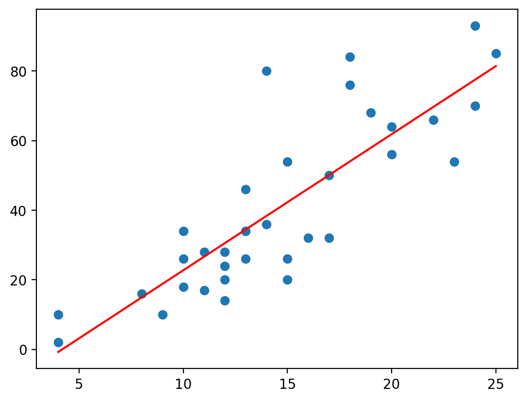
In [182]:

# 선형 회귀식
a = model.coef_
b = model.intercept_
speed = np.linspace(x_train.min(), x_train.max(), 10)
dist = a * speed +b

In [186]:

plt.scatter(x_train, y_train)
plt.plot(speed, dist, color = 'r')
plt.show()

In [216]:

# 예측값, 실젯값 시각화
plt.plot(y_test.values, label = 'Actual')
plt.plot(y_pred, label = 'Predicted')
plt.legend()
plt.show()

In [ ]: