241029
In [8]:
import pandas as pd
import numpy as np
import matplotlib.pyplot as plt
import seaborn as sns
from tqdm.auto import tqdm
import warnings
warnings.filterwarnings('ignore')

import joblib

from sklearn.ensemble import *
from sklearn.model_selection import train_test_split
from sklearn.preprocessing import MinMaxScaler
from sklearn.metrics import *

from sklearn.neighbors import KNeighborsClassifier
from sklearn.tree import DecisionTreeClassifier
from sklearn.model_selection import cross_val_score, GridSearchCV
from sklearn.linear_model import LogisticRegression
from xgboost import XGBClassifier
from lightgbm import LGBMClassifier
1. 지도학습
In [69]:
data01_train = pd.read_csv('data01_train.csv')
data01_train.drop(columns = 'subject', inplace = True)
In [70]:
# LGBM을 위한 열 이름 변경
data01_train.columns = data01_train.columns.str.replace(r'[^\w]', '_', regex=True)
In [71]:
# 데이터 분리
x = data01_train.drop(columns = 'Activity')
y = data01_train['Activity']
x_train, x_val, y_train, y_val = train_test_split(x, y, stratify = y, test_size = 0.3,random_state = 1)
In [75]:
# 정규화
scaler = MinMaxScaler()
x_train = scaler.fit_transform(x_train)
x_val = scaler.transform(x_val)
In [ ]:
# 모델1: Decision Tree
# 모델2: KNN
# 모델3: Random Forest
# 모델4: Logistic Regression
# 모델5: LightGBM
# 모델6: XGBoost
In [38]:
# 모델1: Decision Tree
params = {'max_depth': range(3,30,5)}
model1 = GridSearchCV(DecisionTreeClassifier(random_state = 1),
                                                    params,
                                                    cv = 5,
                                                    scoring = 'accuracy')

model1.fit(x_train, y_train)
print(model1.best_params_)
print(model1.best_score_)
{'max_depth': 8}
0.930756231641284
In [40]:
# 모델1 저장
joblib.dump(model1.best_estimator_, 'model1.pkl')
Out[40]:
['model1.pkl']In [44]:
# 모델2: KNN
params = {'n_neighbors': range(10, 301, 10)}
model2 = GridSearchCV(KNeighborsClassifier(),
                     params,
                     cv = 5,
                     scoring = 'accuracy')
model2.fit(x_train, y_train)
print(model2.best_params_)
print(model2.best_score_)
{'n_neighbors': 10}
0.9494673760454884
In [46]:
# 모델2 저장
joblib.dump(model2.best_estimator_, 'model2.pkl')
Out[46]:
['model2.pkl']In [48]:
# 모델3: Random Forest
params = {'max_depth': range(10, 200, 20)}
model3 = GridSearchCV(RandomForestClassifier(random_state = 1),
                     params,
                     cv = 5,
                     scoring = 'accuracy')

model3.fit(x_train, y_train)
print(model3.best_estimator_)
print(model3.best_score_)
RandomForestClassifier(max_depth=30, random_state=1)
0.9727901709351296
In [50]:
# 모델3 저장
joblib.dump(model3.best_estimator_, 'model3.pkl')
Out[50]:
['model3.pkl']In [77]:
# 모델4: Logistic Regression
model4 = LogisticRegression()
model4.fit(x_train, y_train)
y_pred = model4.predict(x_val)

print(accuracy_score(y_pred, y_val))
print(confusion_matrix(y_pred, y_val))
print(classification_report(y_pred, y_val))
0.9790368271954675
[[335   2   0   0   0   0]
 [  0 292  15   0   0   0]
 [  0  15 311   0   0   0]
 [  0   0   0 298   0   1]
 [  0   0   0   1 237   1]
 [  0   1   0   1   0 255]]
                    precision    recall  f1-score   support

            LAYING       1.00      0.99      1.00       337
           SITTING       0.94      0.95      0.95       307
          STANDING       0.95      0.95      0.95       326
           WALKING       0.99      1.00      0.99       299
WALKING_DOWNSTAIRS       1.00      0.99      1.00       239
  WALKING_UPSTAIRS       0.99      0.99      0.99       257

          accuracy                           0.98      1765
         macro avg       0.98      0.98      0.98      1765
      weighted avg       0.98      0.98      0.98      1765
In [83]:
# 모델4 저장
joblib.dump(model4, 'model4.pkl')
Out[83]:
['model4.pkl']In [79]:
# 모델5: LightGBM
params = {'n_estimators': range(50, 201, 50)}
model5 = GridSearchCV(LGBMClassifier(verbose=-1), params, cv = 5)

model5.fit(x_train, y_train)
print(model5.best_params_)
print(model5.best_score_)
{'n_estimators': 150}
0.9866375089950337
In [85]:
# 모델5 저장
joblib.dump(model5.best_estimator_, 'model5.pkl')
Out[85]:
['model5.pkl']In [93]:
# 모델6: XGBoost

# XGBoost는 숫자형 데이터만 처리 가능
from sklearn.preprocessing import LabelEncoder

le = LabelEncoder()
y_train_label = le.fit_transform(y_train)
y_val_label = le.transform(y_val)


params = {'n_estimators': range(50, 201, 50)}
model6 = GridSearchCV(XGBClassifier(verbose = -1),
                     params,
                     cv = 5,
                     scoring = 'accuracy')

model6.fit(x_train, y_train_label)
print(model6.best_params_)
print(model6.best_score_)
{'n_estimators': 100}
0.9832365015512746
In [95]:
# 모델6 저장
joblib.dump(model6.best_estimator_, 'model6.pkl')
Out[95]:
['model6.pkl']In [ ]:
# 정리
# 모델1: Decision Tree
# 모델2: KNN
# 모델3: Random Forest
# 모델4: Logistic Regression
# 모델5: LightGBM
# 모델6: XGBoost

# 모델 1~5 사용해서 soft voting
In [ ]:
# 앙상블 파이프라인
In [106]:
def pipeline1(filename, target):
    df = pd.read_csv(filename)
    # LGBM을 위한 열 이름 전처리 (json 지원하지 않는 특수 문자 변경)
    df.columns = df.columns.str.replace(r'[^\w]', '_', regex=True)

    # x,y 분리
    x = df.drop(columns = target)
    y = df[target]
    x_train, x_test, y_train, y_test = train_test_split(x, y, stratify = y, test_size = 0.3,random_state = 1)

    # 정규화
    scaler = MinMaxScaler()
    scaler.fit(x_train)
    x_train = scaler.transform(x_train)
    x_test = scaler.transform(x_test)

    model1 = joblib.load('model1.pkl')
    model2 = joblib.load('model2.pkl')
    model3 = joblib.load('model3.pkl')
    model4 = joblib.load('model4.pkl')
    model5 = joblib.load('model5.pkl')

    # 보팅 모델 선언
    estimators = [('DT', model1),
                  ('KNN', model2),
                  ('RF', model3),
                  ('LR', model4),
                  ('LGBM', model5)]

    model_voting = VotingClassifier(estimators=estimators, voting = 'soft')

    # 학습하기
    model_voting.fit(x_train, y_train)

    # 예측하기
    y_pred = model_voting.predict(x_test)

    acc_score = accuracy_score(y_test, y_pred)
    conf_matrix = confusion_matrix(y_test, y_pred)
    class_report = classification_report(y_test, y_pred)

    joblib.dump(model_voting,'model_pipeline1.pkl')

    return acc_score, conf_matrix, class_report
In [112]:
accuracy, confusion, report = pipeline1('data01_test.csv', 'Activity')
print(accuracy)
print(confusion)
print(report)
0.9570135746606335
[[88  0  0  0  0  0]
 [ 3 62 11  0  0  0]
 [ 0  0 86  0  0  0]
 [ 0  0  0 67  1  0]
 [ 0  0  0  2 57  0]
 [ 0  0  0  0  2 63]]
                    precision    recall  f1-score   support

            LAYING       0.97      1.00      0.98        88
           SITTING       1.00      0.82      0.90        76
          STANDING       0.89      1.00      0.94        86
           WALKING       0.97      0.99      0.98        68
WALKING_DOWNSTAIRS       0.95      0.97      0.96        59
  WALKING_UPSTAIRS       1.00      0.97      0.98        65

          accuracy                           0.96       442
         macro avg       0.96      0.96      0.96       442
      weighted avg       0.96      0.96      0.96       442
In [ ]:
2. 비지도 학습
In [17]:
from sklearn.cluster import KMeans
from yellowbrick.cluster import KElbowVisualizer
In [18]:
# standard scaling 된 데이터 data_sc.csv 불러오기
data = pd.read_csv('data_sc.csv')
data.tail()
Out[18]:
AGE고용상태Willingness to pay/Stay상품타입교육수준소득월 납입액타 상품 보유 현황총지불금액거주지사이즈자동차1199511996119971199811999
| -1.853401 | 0.772120 | 2.224522 | -0.313685 | -0.366062 | 1.071545 | -0.708232 | -0.247307 | -0.809917 | -0.340235 | -0.318628 |
| -0.070427 | 0.772120 | -0.703830 | -0.313685 | -0.366062 | -0.547511 | -0.472671 | -1.078127 | -0.188373 | -0.340235 | -0.318628 |
| -0.070427 | -1.295136 | 0.025735 | -0.313685 | -0.366062 | -1.242413 | -0.237111 | -0.247307 | 1.230306 | -0.340235 | -0.318628 |
| 0.821059 | 0.772120 | -0.066542 | -0.313685 | -0.366062 | -0.536698 | -0.001551 | 0.583512 | 0.887482 | 2.939142 | -0.318628 |
| -0.070427 | -1.295136 | -0.774479 | -0.313685 | -0.366062 | -1.242413 | -0.472671 | -1.078127 | -0.221820 | -0.340235 | -0.318628 |
In [26]:
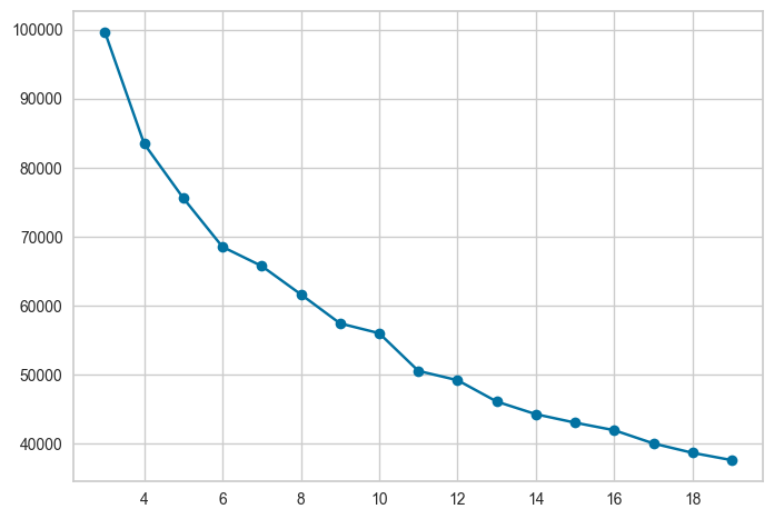
# 몇개로 군집화 할지 시각화로 판단
kvalues = range(3, 20)
inertias = list()

for k in kvalues:
    model = KMeans(n_clusters = k, n_init = 'auto', random_state =1)
    model.fit(data)
    inertias.append(model.inertia_)

plt.plot(kvalues, inertias, marker = 'o')
plt.show()
In [38]:
# Elbow Method 활용 k 결정
model = KMeans(random_state = 1, n_init = 'auto')
Elbow_M = KElbowVisualizer(model,k=(2,21))
Elbow_M.fit(data)
Elbow_M.show()
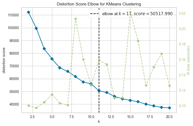
Out[38]:
<Axes: title={'center': 'Distortion Score Elbow for KMeans Clustering'}, xlabel='k', ylabel='distortion score'>In [41]:
#???
In [51]:
# 데이터 불러오기
data0 =pd.read_csv('customers_seg.csv')
data0.drop(columns = ['CID'], inplace  =True)
In [53]:
# 6개의 cluster
model_B =KMeans(n_clusters = 6, n_init = 'auto')

model_B.fit(data)

cluster = model_B.predict(data)
cluster
Out[53]:
array([1, 2, 1, ..., 1, 4, 1])In [59]:
# cluster를 데이터프레임으로 만들고 붙이기
# result에는 cluster가 포함
cluster = pd.DataFrame(cluster, columns = ['cluster'])
result = pd.concat([data0, cluster], axis = 1)
result['cluster'] = pd.Categorical(result['cluster'] )

result.to_csv('result_my.csv', index = False)
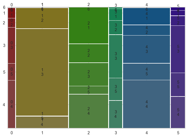
In [67]:
# AGE 열 파악하기
feature = 'AGE'

df = pd.crosstab([result[feature]], result['cluster'], margins=True)

# pro_df 확인
display(df)

# 시각화
from statsmodels.graphics.mosaicplot import mosaic
mosaic(result.sort_values('cluster'), ['cluster', feature])
plt.show()
cluster012345AllAGE123456All
| 43 | 0 | 823 | 87 | 461 | 40 | 1454 |
| 38 | 621 | 421 | 106 | 273 | 79 | 1538 |
| 154 | 2623 | 524 | 330 | 753 | 391 | 4775 |
| 206 | 355 | 773 | 212 | 1314 | 264 | 3124 |
| 71 | 0 | 177 | 169 | 447 | 193 | 1057 |
| 2 | 0 | 1 | 11 | 11 | 27 | 52 |
| 514 | 3599 | 2719 | 915 | 3259 | 994 | 12000 |
In [ ]:
'KT AIVLE > Daily Review' 카테고리의 다른 글
| 241031 (0) | 2024.10.31 |
|---|---|
| 241030 (0) | 2024.10.30 |
| 241021 ~ 241022 (0) | 2024.10.28 |
| 241018 (0) | 2024.10.20 |
| 241017 (0) | 2024.10.17 |