241101
In [1]:
import pandas as pd
import numpy as np
import matplotlib.pyplot as plt
import seaborn as sns

from sklearn.model_selection import train_test_split
from sklearn.metrics import *
from sklearn.preprocessing import StandardScaler, MinMaxScaler

from keras.models import Sequential
from keras.layers import Dense, Flatten, Input
from keras.backend import clear_session
from keras.optimizers import Adam
from keras.datasets import mnist, fashion_mnist
1. 다중 분류 (MNIST)
In [2]:
# 데이터 불러오기
(x_train, y_train), (x_val, y_val) = mnist.load_data()
Downloading data from https://storage.googleapis.com/tensorflow/tf-keras-datasets/mnist.npz
11490434/11490434 ━━━━━━━━━━━━━━━━━━━━ 1s 0us/step
In [3]:
x_train.shape, y_train.shape
Out[3]:
((60000, 28, 28), (60000,))In [5]:
# 데이터 2차원으로 펼치기
x_train = x_train.reshape(60000,-1)
x_val = x_val.reshape(10000,-1)

x_train.shape, x_val.shape
Out[5]:
((60000, 784), (10000, 784))In [6]:
# scaling
x_train = x_train / 255.
x_val = x_val / 255.
In [9]:
# 모델링
nfeatures = x_train.shape[1]

clear_session()

model = Sequential([Input(shape = (nfeatures, )),
                    Dense(128, activation = 'relu'),
                    Dense(64 ,activation = 'relu'),
                    Dense(32, activation = 'relu'),
                    Dense(10, activation = 'softmax')])

# 컴파일, 학습
model.compile(optimizer = Adam(learning_rate = 0.001), loss = 'sparse_categorical_crossentropy')
hist = model.fit(x_train, y_train, epochs = 50, validation_split = .2, verbose = 0).history
In [13]:
# 시각화
plt.plot(hist['loss'], label = 'train_err', marker = '.')
plt.plot(hist['val_loss'], label = 'val_err', marker = '.')
plt.legend()
plt.grid()
plt.show()
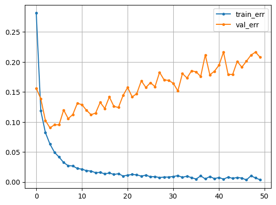
In [14]:
# 과적합 발생
In [14]:
2. Early Stopping
In [20]:
from keras.callbacks import EarlyStopping
In [15]:
path = "https://raw.githubusercontent.com/DA4BAM/dataset/master/overfit_sample.csv"
data = pd.read_csv(path)
data.tail()
Out[15]:
target012345678...290291292293294295296297298299245246247248249
| 1 | -0.068 | -0.184 | -1.153 | 0.610 | 0.414 | 1.557 | -0.234 | 0.950 | 0.896 | ... | 1.492 | 1.430 | -0.333 | -0.200 | -1.073 | 0.797 | 1.980 | 1.191 | 1.032 | -0.402 |
| 0 | -0.234 | -1.373 | -2.050 | -0.408 | -0.255 | 0.784 | 0.986 | -0.891 | -0.268 | ... | -0.996 | 0.678 | 1.395 | 0.714 | 0.215 | -0.537 | -1.267 | -1.021 | 0.747 | 0.128 |
| 0 | -2.327 | -1.834 | -0.762 | 0.660 | -0.858 | -2.764 | -0.539 | -0.065 | 0.549 | ... | -1.237 | -0.620 | 0.670 | -2.010 | 0.438 | 1.972 | -0.379 | 0.676 | -1.220 | -0.855 |
| 1 | -0.451 | -0.204 | -0.762 | 0.261 | 0.022 | -1.487 | -1.122 | 0.141 | 0.369 | ... | 0.729 | 0.411 | 2.366 | -0.021 | 0.160 | 0.045 | 0.208 | -2.117 | -0.546 | -0.093 |
| 0 | 0.725 | 1.064 | 1.333 | -2.863 | 0.203 | 1.898 | 0.434 | 1.207 | -0.015 | ... | -1.028 | 1.081 | 0.607 | 0.550 | -2.621 | -0.143 | -0.544 | -1.690 | -0.198 | 0.643 |
5 rows × 301 columns
In [16]:
# 데이터분할 : x, y
target = 'target'
x = data.drop(columns = target)
y = data[target]

# 데이터분할 : train, validation
x_train, x_val, y_train, y_val = train_test_split(x, y, test_size=0.3, random_state = 1)
In [17]:
# 스케일링
scaler = MinMaxScaler()
x_train = scaler.fit_transform(x_train)
x_val = scaler.transform(x_val)
In [18]:
# 모델링
nfeatures = x_train.shape[1]

clear_session()

model = Sequential([Input(shape = (nfeatures, )),
                    Dense(128, activation = 'relu'),
                    Dense(64, activation = 'relu'),
                    Dense(32, activation = 'relu'),
                    Dense(1, activation = 'sigmoid')])

# 컴파일, 학습
model.compile(optimizer = Adam(learning_rate = 0.001), loss = 'binary_crossentropy')
hist = model.fit(x_train, y_train, epochs = 50, verbose = 0, validation_split = 0.2).history
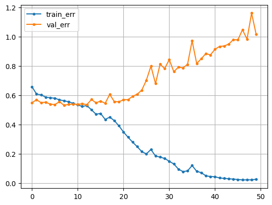
In [19]:
# 시각화
plt.plot(hist['loss'], label = 'train_err', marker = '.')
plt.plot(hist['val_loss'], label = 'val_err', marker = '.')
plt.legend()
plt.grid()
plt.show()
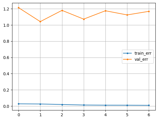
In [21]:
# early stopping 설정
min_de = 0.001
pat = 5

es = EarlyStopping(monitor = 'val_loss', min_delta = min_de, patience = pat)

# 학습
hist = model.fit(x_train, y_train, epochs = 50, validation_split = 0.2,
                 callbacks = [es]).history

# 시각화
plt.plot(hist['loss'], label = 'train_err', marker = '.')
plt.plot(hist['val_loss'], label = 'val_err', marker = '.')
plt.legend()
plt.grid()
plt.show()
Epoch 1/50
5/5 ━━━━━━━━━━━━━━━━━━━━ 0s 43ms/step - loss: 0.0286 - val_loss: 1.2123
Epoch 2/50
5/5 ━━━━━━━━━━━━━━━━━━━━ 0s 8ms/step - loss: 0.0323 - val_loss: 1.0409
Epoch 3/50
5/5 ━━━━━━━━━━━━━━━━━━━━ 0s 7ms/step - loss: 0.0218 - val_loss: 1.1792
Epoch 4/50
5/5 ━━━━━━━━━━━━━━━━━━━━ 0s 7ms/step - loss: 0.0137 - val_loss: 1.0717
Epoch 5/50
5/5 ━━━━━━━━━━━━━━━━━━━━ 0s 7ms/step - loss: 0.0115 - val_loss: 1.1745
Epoch 6/50
5/5 ━━━━━━━━━━━━━━━━━━━━ 0s 7ms/step - loss: 0.0112 - val_loss: 1.1232
Epoch 7/50
5/5 ━━━━━━━━━━━━━━━━━━━━ 0s 8ms/step - loss: 0.0095 - val_loss: 1.1672
In [ ]:
3. Dropout
In [22]:
from keras.layers import Dropout
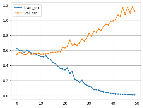
In [23]:
# 모델링
nfeatures = x_train.shape[1]

clear_session()

model1 = Sequential( [Input(shape = (nfeatures,)),
                      Dense(128, activation= 'relu'),
                      Dense(64, activation= 'relu'),
                      Dense(32, activation= 'relu'),
                      Dense(1, activation= 'sigmoid')] )

# 컴파일, 학습
model1.compile(optimizer= Adam(learning_rate = 0.001), loss='binary_crossentropy')
hist1 = model1.fit(x_train, y_train, epochs = 50, validation_split=0.2, verbose = 0).history

# 시각화
plt.plot(hist1['loss'], label = 'train_err', marker = '.')
plt.plot(hist1['val_loss'], label = 'val_err', marker = '.')
plt.legend()
plt.grid()
plt.show()
In [24]:
# dropout 모델링
clear_session()

model2 = Sequential( [Input(shape = (nfeatures,)),
                      Dense(128, activation= 'relu'),
                      Dropout(0.4),
                      Dense(64, activation= 'relu'),
                      Dropout(0.4),
                      Dense(32, activation= 'relu'),
                      Dropout(0.4),
                      Dense(1, activation= 'sigmoid')] )

# 컴파일, 학습
model2.compile(optimizer= Adam(learning_rate = 0.001), loss='binary_crossentropy')
hist2 = model2.fit(x_train, y_train, epochs = 50, validation_split=0.2, verbose = 0).history

# 시각화
plt.plot(hist2['loss'], label = 'train_err', marker = '.')
plt.plot(hist2['val_loss'], label = 'val_err', marker = '.')
plt.legend()
plt.grid()
plt.show()
In [ ]: